2- Creating a baseline with EnergyLab

There are 2 ways to create baselines with EnergyLab:

1. The automated baseline
2. The customized baseline.

1. Creating an automatic baseline

This is the quickest and most efficient way of modeling a reference situation, based on consumption data and influential parameters.

It simply requires :

• The choice of a reference period,
• The target variable,
• Potential influential parameters.
• Model frequency (hourly, daily, etc.).

From the Data Sources area, click on “Add” then “Simplified model”. 

The video below takes you through the various steps: 


 
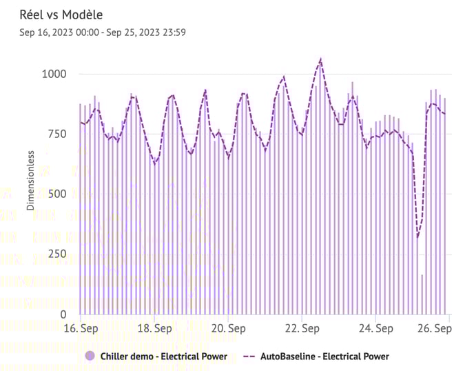
You can then find your automatic baseline in Data Sources and use it in a widget like any other series.
Example with the template created from the video above:

---

2. Creating a custom baseline

The custom baseline is the most precise and adaptable way of defining and modeling a reference situation. It allows you to explore the data to best define the reference period and influential factors.

Create a model

Go to the EnergyLab workspace and click on “ + New model ” at the top of your screen:

Name your workflow, fill in the required information and click Apply:

• Title (must be unique).
• Project to link (click “+” to add projects)
• Tags (click “+” to add tags)
• Workflow type: for the moment, only the “Empty” type is available.
  
  

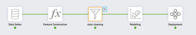
There are 5 steps to template creation:

• A) Data retrieval
• B) Data construction
• C) Data cleansing
• D) Modeling
• E) Deployment

For each of the 5 steps, you can view the data used. 

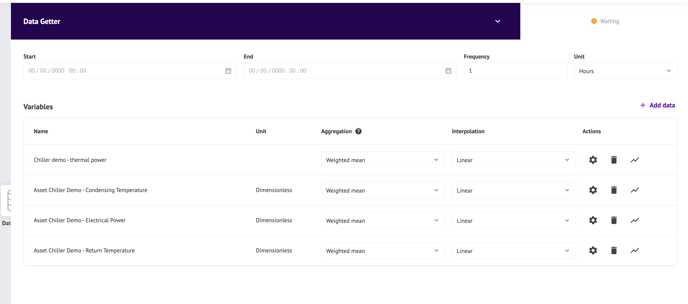
A) Data retrieval

In this step, you will retrieve the data relevant to your analysis from the data sources on your METRON platform.

Instructions :

• Select the start and end date and time of the data you wish to retrieve.
• Select the frequency of your point collection (also known as granularity).
• Select the different series whose data you wish to retrieve.
• For each variable: select aggregation and interpolation.

B) Data cleaning

In this block, you can clean up your data by removing outliers (i.e. points representing erroneous measurements or isolated maintenance or incident events).

To do this, you can create rules to implement physical constraints (e.g. energy >0). You can also graphically select from a point cloud those you wish to keep or remove.

Instructions :

Choose a data cleansing method: 

• With rules :
  • Select a variable, an operator and a second operand (value or variable).
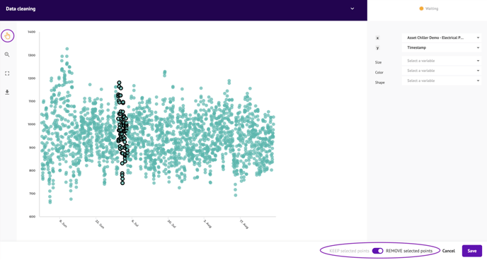
• From a point cloud: Use graphic selection :
  • Select the different variables for the X/Y axes.
  • Add additional variables for color, shape and size.
  • Select the points you wish to keep or delete with the selection tool.
  • To select several areas of the graph, hold down the SHIFT key and click on the different areas you wish to keep or delete.
  • You can choose to keep or delete the points selected in the bottom right-hand corner.

• Automatic cleaning:
  • Let our algorithm clean up the data for you.

C) Data construction

In this block, you can enrich your dataset selected in the first step, by combining existing variables to create new ones.

Instructions :
On the left, you can import and name the variables you want to use in your calculation.

On the right, you can name the result of each calculation.

Use the calculation panel to define the formula for your new variable (see below), including :

• Arithmetic operators +, -, *, /, ** (power), % (modulo), // (floor division).
• Comparison operators <, >, <=, >=,!=, ==.
• Boolean operators | (or), & (and), and ~ (not)
• Mathematical functions sin, cos, exp, log, expm1 (exp minus one), log1p (log(1+x)), sqrt, sinh, cosh, tanh, arcsin, arccos, arctan, arccosh, arcsinh, arctanh, abs and arctan2

Example: If you want to create the exponential of energy + the log of production, you'd use “exp(energy) + log(production)”. 

A Boolean of consumption greater than 10 and production less than 2000 would be “consumption > 10 & production < 2000”.

D) Modeling

In this block, you can select the model(s) you wish to train.

Instruction :

• Select model(s): you can choose 1, 2 or all 3 models to compare and define which one will be the most suitable, and preview the results.
  • Linear regression: this model is selected by default.
  • Random forest: to model non-linear phenomena.
  • kNN: for direct comparison with similar points.
• Select the target variable to be predicted:
  • Ex: the power consumption of a UES.
• Select the characteristic variables you wish to use for your prediction
  • Ex: influential factors identified for this SEU.
• Select your method for separating training and test data:
  • Ratio: The first X% of the data will be used for training, the rest for testing. 
  • Date/time: Data preceding the date/time will be used for training, and data following it will be used for testing.
  • Ex: We can use the year 2023 as the training period and the 2024 data for testing. 
• Start calculating the models, then compare their performance. 

To find out more, see Interpreting model results (coming soon).

E) Deployment

In this block, you will save your model and publish it on the platform. You'll find it in Data sources. Once a model has been published, predictions will be calculated live as long as input data is available. 

Instruction:

• Choose a model from those trained in the previous block.
• Enter a name for your model.
• Select a date from which to calculate the history.